My previous post. . All my code can be found on github (7_Basic_Neural_Network.ipynb)
The Brain!
Now that we know how to train a data graph lets create our first basic Neural Network (NN). A Neural network is:
- A digital network inspired by neurons in the brain.
- Has a number of input nodes where data flows IN.
- A number of output nodes where data flows OUT (Results).
- A number of hidden nodes organised into layers that connect the input and output nodes.
- Networks with only a few hidden layers are called shallow and networks with many hidden layers are called deep.
- The connection between nodes have weights and biases values that change during training.
- The arrangement of the nodes is called the network architecture and there are many different arrangements as can be seen here.

3 input nodes. 4 hidden nodes in 1 layer and 2 output nodes
Neuron
At a basic level each Node in the network is meant to represent a Neuron in the brain. It takes many inputs and generates an output.

As you can see each input to the node is multiplied by the weight along that edge. A bias value is then added and then this is passed through an activation function. I will go into activation functions at a later time.
This calculates for each node:
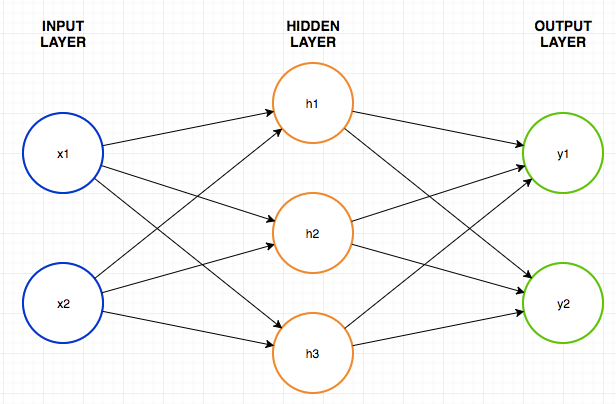
Network
When the nodes are arranges in a network they generally take the following form. This is called a feed forward network. This is because the data feeds from left to right through the network and is one of the simplest neural network architectures.

When we label all of the weights and biases for each of the nodes and edges of the network this looks like this:

Although this looks complicated we can thankfully represent this in the form of matrices and also the algebra in the form of matrix multiplications.
The tensorflow website explains this well. (Softmax as their activation function)

Which becomes:

that can be expressed as:
![]()
Code – Generate Data
We will train the network the in a similar way to the previous lesson by using labeled training data. As the network trains the values for the weights and biases are changed in an attempt the make the inputs match the outputs.
I will aim to create a system that converts binary input (base 2 number) into decimal output (base 10 number).
Lets create some training data.
# Generate Sample Points

IN_binary =  [[0, 0, 0, 0],    #0
              [0, 0, 0, 1],    #1
              [0, 0, 1, 0],    #2
              [0, 0, 1, 1],    #3
              [0, 1, 0, 0],    #4
              [0, 1, 0, 1],    #5
              [0, 1, 1, 0],    #6
              [0, 1, 1, 1],    #7
              [1, 0, 0, 0],    #8
              [1, 0, 0, 1],    #9
              [1, 0, 1, 0],    #10
              [1, 0, 1, 1],    #11
              [1, 1, 0, 0],    #12
              [1, 1, 0, 1],    #13
              [1, 1, 1, 0],    #14
              [1, 1, 1, 1]]    #15

#              0, 1, 2, 3, 4, 5, 6, 7, 8, 9,10,11,12,13,14,15,
OUT_dec =    [[1, 0, 0, 0, 0, 0, 0, 0, 0, 0, 0, 0, 0, 0, 0, 0],
              [0, 1, 0, 0, 0, 0, 0, 0, 0, 0, 0, 0, 0, 0, 0, 0],
              [0, 0, 1, 0, 0, 0, 0, 0, 0, 0, 0, 0, 0, 0, 0, 0],
              [0, 0, 0, 1, 0, 0, 0, 0, 0, 0, 0, 0, 0, 0, 0, 0],
              [0, 0, 0, 0, 1, 0, 0, 0, 0, 0, 0, 0, 0, 0, 0, 0],
              [0, 0, 0, 0, 0, 1, 0, 0, 0, 0, 0, 0, 0, 0, 0, 0],
              [0, 0, 0, 0, 0, 0, 1, 0, 0, 0, 0, 0, 0, 0, 0, 0],
              [0, 0, 0, 0, 0, 0, 0, 1, 0, 0, 0, 0, 0, 0, 0, 0],
              [0, 0, 0, 0, 0, 0, 0, 0, 1, 0, 0, 0, 0, 0, 0, 0],
              [0, 0, 0, 0, 0, 0, 0, 0, 0, 1, 0, 0, 0, 0, 0, 0],
              [0, 0, 0, 0, 0, 0, 0, 0, 0, 0, 1, 0, 0, 0, 0, 0],
              [0, 0, 0, 0, 0, 0, 0, 0, 0, 0, 0, 1, 0, 0, 0, 0],
              [0, 0, 0, 0, 0, 0, 0, 0, 0, 0, 0, 0, 1, 0, 0, 0],
              [0, 0, 0, 0, 0, 0, 0, 0, 0, 0, 0, 0, 0, 1, 0, 0],
              [0, 0, 0, 0, 0, 0, 0, 0, 0, 0, 0, 0, 0, 0, 1, 0],
              [0, 0, 0, 0, 0, 0, 0, 0, 0, 0, 0, 0, 0, 0, 0, 1]]
Our input will be a binary array. Our output will have 16 nodes each representing a different digit.
CODE – Create Neural Network
Lets assign some parameters that describe the architecture of the network.
#Network Parameters
INPUTS = 4
HIDDEN_1 = 20
OUTPUTS = 16

#Hyper Parameters
learning_rate = 0.1
CODE – Placeholders
Now to pass this training data into the system we need placeholders same as the previous lesson
#Use placeholders to pass our input and output data into the system
x_data = tf.placeholder(dtype=tf.float32,shape=[None, INPUTS],name="input")
y_data = tf.placeholder(dtype=tf.float32,shape=[None, OUTPUTS],name="output")
Note the shape section. The None indicates how many items we will be training on at one time. None indicates any number of training items. It is often more efficient to train on multiple training samples at a time called batch training.
CODE – Variables
We then need to create Variables to hold our weights and biases.
- Weights between the inputs and hidden layer
- Weights between the hidden layer and output units.
- Biases for the Hidden Layer
- Biases for the output layer.
These will all be initialized with random data using the tensorflows tf.random_normal function. We could have also used numpy as in the previous less.
#input to hidden
weight1 = tf.random_normal([INPUTS, HIDDEN_1], mean=0.5, stddev=0.7)
weight1 = tf.Variable(weight1, name='W1')

bias1 = tf.random_normal([HIDDEN_1], mean=0.5, stddev=0.7)
bias1 = tf.Variable(bias1, name='B1')

weight2 = tf.random_normal([HIDDEN_1, OUTPUTS], mean=0.5, stddev=0.7)
weight2 = tf.Variable(weight2, name='W2')

bias2 = tf.random_normal([OUTPUTS], mean=0.5, stddev=0.7)
bias2 = tf.Variable(bias2, name='B2')
Then we will add in the matrix multiplications that connect all of the layers together.
#input to hidden
hidden1 = tf.nn.relu(tf.matmul(x_data, weight1) + bias1)

#hidden to output
y = tf.matmul(hidden1, weight2) + bias2
The outputs of the system need to undergo a softmax activation function. This is used for multiclass logistic regression. It turns the total output of the system to equal 1.
#apply final activation
result = tf.nn.softmax(y)
CODE – Training
Now we need to undergo our normal training system.
- Define the loss
- Define the optimiser
- Train on Data.
loss = tf.reduce_mean(
tf.nn.softmax_cross_entropy_with_logits(logits=y, labels=y_data))
This is slightly different from using Mean Squared Error.
We will use the AdamOptimiser. Tensorflow has a number of different optimizers. A good discussion with a nice animation on the differences can be found here.
optimizer = tf.train.AdamOptimizer(learning_rate)
train = optimizer.minimize(loss)
To train on data we will need to pass in the training data using a feed_dictionary
epochs = 2000
display_epochs = 100

for step in range(epochs):
    result = session.run([train,loss],feed_dict={x_data: IN_binary, y_data: OUT_dec})
    if step % display_epochs == 0:
        print("Step: %d error: %g "%(step,result[1]))
This is very similar to previous lessons training.
Lets run the system and see how it performs.

The error rate looks really good except we probably could have stopped training before 100 steps let alone 2000.
Lets add in code to stop training when our error rate gets to an acceptable level ( <0.005 ). Lets rerun and see.

It now exits after 36 steps.
Graph code
Now that the system is trained we can have a look at its performance.
For this we will input data into the data graph and output a bar graph to show what the system believes the correct output should be.
Firstly the following generates a matplotlib bar graph from an array of values.
def bar_graph(label,res):
    print(label)
    y = res[0]
    N = len(y)
    x = range(N)
    width = 1/1.5
    plt.bar(x, y, width, color="blue")
    plt.show()
We will then pass in all of the different options to see how the system performs.
#Test outputs
bar_graph("0 with softmax",session.run(result, feed_dict={x_data: [[ 0, 0, 0, 0]]}))
bar_graph("0 without softmax",session.run(y, feed_dict={x_data: [[ 0, 0, 0, 0]]}))#

bar_graph("1",session.run(result, feed_dict={x_data: [[ 0, 0, 0, 1]]}))
bar_graph("2",session.run(result, feed_dict={x_data: [[ 0, 0, 1, 0]]}))
bar_graph("3",session.run(result, feed_dict={x_data: [[ 0, 0, 1, 1]]}))
bar_graph("4",session.run(result, feed_dict={x_data: [[ 0, 1, 0, 0]]}))
bar_graph("5",session.run(result, feed_dict={x_data: [[ 0, 1, 0, 1]]}))
bar_graph("6",session.run(result, feed_dict={x_data: [[ 0, 1, 1, 0]]}))
bar_graph("7",session.run(result, feed_dict={x_data: [[ 0, 1, 1, 1]]}))
bar_graph("8",session.run(result, feed_dict={x_data: [[ 1, 0, 0, 0]]}))
bar_graph("9",session.run(result, feed_dict={x_data: [[ 1, 0, 0, 1]]}))
bar_graph("10",session.run(result, feed_dict={x_data: [[ 1, 0, 1, 0]]}))
bar_graph("11",session.run(result, feed_dict={x_data: [[ 1, 0, 1, 1]]}))
bar_graph("12",session.run(result, feed_dict={x_data: [[ 1, 1, 0, 0]]}))
bar_graph("13",session.run(result, feed_dict={x_data: [[ 1, 1, 0, 1]]}))
bar_graph("14",session.run(result, feed_dict={x_data: [[ 1, 1, 1, 0]]}))
bar_graph("15",session.run(result, feed_dict={x_data: [[ 1, 1, 1, 1]]}))
softmax vs non softmax output. This illustrates what the softmax function does for the 0 input.

So you can now test the trained network.

Next we will apply this system to the MNIST dataset for handwriting digits.