My previous post. . All my code can be found on github (6_TrainingWithLinearRegression.ipynb)
The aim of a Neural Network is to get the output for the model to match the expected output of a system. The difference between these values is the error. We want to minimise this.
Training is a 3 step process
- Define a LOSS FUNCTION – how accurate the model is
- Define an OPTIMISER – how to make the model more accurate
- Train it with data – to minimise the loss.
To demonstrate training we will implement Linear Regression. This will bring together some of the previous lessons and introduce some new topics.
Linear Regression
Linear regression is a line of best fit to a set of data points. The line can be expressed in the form of Y = Ax + B, where A and B are variables. The aim is to find the values for A and B such that the line fits the data nicely like below.

There are other forms of Regressions such as Polynomial:

Create some Test Data
We will start by creating some fake data that we will aim to fit to.
First lets create our own line. We will be using the library matplotlib to plot data to the screen.
#import libraries
import numpy as np
import tensorflow as tf

import matplotlib.pyplot as plt

%matplotlib inline
Matplotlib is python graph plotting library. %matplotlib inline helps display the graphs in jupyter.
Lets create our fake data. We set our two variables to find A = 3.5 and B = 2. Create an input range for X and create the linear function for Y.
# Generate Samle Points
a_data=3.5
b_data=2

x_data = np.random.rand(100).astype(np.float32)
y_data = x_data * a_data + b_data


plt.plot(x_data,y_data)
plt.ylabel('Y')
plt.xlabel('X')
plt.show()

Now we have a line we need to turn it into points. We should also add some noise to replicate a real life data source.
# Add Noise
def add_noise(y):
   return y+np.random.normal(loc=0.0, scale=0.5)
y_data = map(add_noise,y_data)
Now if we plot the X and Y points as a scatter plot we get.

Create Data Graph
Now we have our training data lets create our data graph we want to solve.
We will need:
- 2 variables A and B to train.
- A loss function
- An optimiser
- A trainer
Now lets feed in the training data we generated and hopefully it should find the values of A = 3.5 and B = 2.
# to Solve
a = tf.Variable(1.0, name = 'A')
b = tf.Variable(1.0, name = 'B')

y = a * x_data + b
I have initialised the variables with 1.0 but it is normal practice to initialise them with random values e.g.
a = tf.Variable(np.random.normal(loc=1.0, scale=1.0), name = 'A')
The loss function is the difference between the output (y) and the expected output (y_data). We use Mean Squared Error (MSE) which is a common loss function described here.
loss = tf.reduce_mean(tf.square(y - y_data))
The optimiser we will use is Gradient Descent. You will normally use a variant of Gradient Descent. The learning rate is how fast it will adjust the values.
learning_rate = 0.1
optimizer = tf.train.GradientDescentOptimizer(learning_rate)
Then the training function is simply aiming to minimise the loss.
train = optimizer.minimize(loss)
Then lets run the training data. We run this again and again. Each training step of the training data is called an Epoch. Each time it runs the gradient descent algorithm alters the variables to minimise the loss function.
Remember to initialise variables first.
init = tf.global_variables_initializer()
session = tf.Session()
session.run(init)
Lets run the trainer 10 times and see how it goes.
for step in range(10):
    result = sess.run(train)
    print(sess.run([a,b,loss]))
After each training run we print out the values of a, b and the loss value. We hope A approaches 3.5, B approaches 2 and the loss approaches 0.

A is headed towards 3.5, B is headed towards 2 and the loss function is headed towards 0. But it looks like this is going to take a lot more Epochs.
Lets clean up the code a bit, change Epochs to 400 and now only display the outputs every 40 items.

We end up with values of A = 3.63, B = 1.93 and a loss of 0..31. Which is nice and close.
It doesn’t exactly match the initial values because of the random noise we added to the training data.
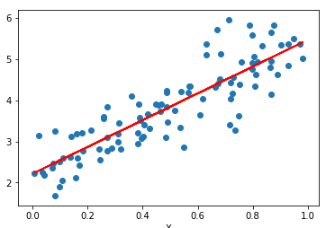
Now how does this look plotted against our training data? Lets plot the training data against the line we trained

And lets finally close the session
session.close()