My previous post. . All my code can be found on github (8_MNIST_1.ipynb)
MNIST
The MNIST dataset consists of images of handwritten digits comprising of 55,000 training examples, 10,000 training examples and 5000 validation examples. MNIST is an extremely popular image dataset to work on because its easy to get started on and you can try different approaches that increase the accuracy of your solution. It originates from http://yann.lecun.com/exdb/mnist/
Data Acquisition
First lets download the data. We will store this in /tmp/data/ folder. The MNIST dataset is so popular that Tensorflow includes helper functions to download it as part of the library. We will copy the Tensorflow official MNIST tutorial code to download the files from here. Each part will be stored in X_Type and Y_Type variables.

The data is split into training, validation and test data. We use the training and validation data during training and the test data only to test our final solution. We want to avoid an issue called overfitting. This is when the system begins to memorise the training data instead of learning a more generalised solution. If the accuracy of the system on the training data increases but the accuracy over the validation data (a dataset which it hasn’t been trained on) also doesn’t increase this indicates overfitting and you should stop training.
This is what the data actually looks like.

As you can see the Y_train[0] represents the number 7 because all other labels are value = 0 and 7 has value 1. The image training data is a 28 x 28 pixel 2D array flattened down to one long 784 long array. This removes the 2D structure of the data. Each pixel in the 784 long float array is between 0 and 1 in greyscale intensity. Therefore X_Train[0] is a giant 784 long float array.
To visualise what the actual MNIST images look like i will make a simple matplotlib function to take an input array and output the image. It has an optional inverse command.
def display_mnist(input_array, invert = False):
    first_image = []
    if invert:
        first_image = np.array(input_array*255, dtype='uint8')
    else:
        first_image = np.array((1-input_array)*255, dtype='uint8')

    pixels = first_image.reshape((28, 28))
    plt.imshow(pixels, cmap='gray')
    plt.show()

# Call function on different training data
display_mnist(X_train[1],True)
display_mnist(X_train[1])

display_mnist(X_train[2])
display_mnist(X_train[3])
display_mnist(X_train[4])
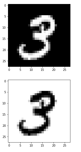
Here is a 3 and an inversed 3.
 And a 6 and 1. The 6 is not very legible.

Basic NN
We will reuse the same model from the previous lesson with some minor modifications.
Firstly we now have 784 inputs for each pixel of data and 10 outputs for the digits 0 to 9. To begin with i will set the hidden layer to 200 nodes and a learning rate of 0.001.
#Network Parameters
INPUTS = 784       # 28 x 28 = 784 input pixels
HIDDEN_1 = 200      # we will start with a NN with 1 hidden layer and 40 nodes.
OUTPUTS = 10       # 10 possible outputs - 0->9

#Training Parameters
epochs = 1000
display_epochs = 50
batch_size = 1000
learning_rate = 0.001
Same placeholders as before
#Use placeholders to pass our input and output data into the system
x_data = tf.placeholder(dtype=tf.float32,shape=[None, INPUTS],name="input")
y_data = tf.placeholder(dtype=tf.float32,shape=[None, OUTPUTS],name="output")
I will reuse the same code for the Neural Network and use the same loss function and optimizer.
#Structure
weight1 = tf.random_normal([INPUTS, HIDDEN_1], mean=0.5, stddev=0.7)
weight1 = tf.Variable(weight1, name='W1')

bias1 = tf.random_normal([HIDDEN_1], mean=0.5, stddev=0.7)
bias1 = tf.Variable(bias1, name='B1')

weight2 = tf.random_normal([HIDDEN_1, OUTPUTS], mean=0.5, stddev=0.7)
weight2 = tf.Variable(weight2, name='W2')

bias2 = tf.random_normal([OUTPUTS], mean=0.5, stddev=0.7)
bias2 = tf.Variable(bias2, name='B2')

#input to hidden
hidden1 = tf.nn.relu(tf.matmul(x_data, weight1) + bias1)

#hidden to output
y = tf.matmul(hidden1, weight2) + bias2

#apply final activation
result = tf.nn.softmax(y)

#loss and training
loss = tf.reduce_mean(tf.nn.softmax_cross_entropy_with_logits(logits=y, labels=y_data))

optimizer = tf.train.AdamOptimizer(learning_rate)
train = optimizer.minimize(loss)
Note nn.softmax_cross_entropy_with_logits performs the nn.softmax operation so we don’t need to explicitly call it.
Training
for step in range(epochs):
    #get a random batch of data
    batch_x, batch_y = mnist.train.next_batch(batch_size)

    #run the training and the loss
    out_training , out_loss = session.run([train,loss],feed_dict={x_data: batch_x, y_data: batch_y})


    if step % display_epochs == 0:
        print("Step: %d error: %g "%(step,out_loss))
The training looks the same as the previous lesson except for the following line:
batch_x, batch_y = mnist.train.next_batch(batch_size)
Instead of training the network on the entire 55,000 training examples we use a random sample, a batch of training data. In this case we use 1000 items. This method of using batches instead of the complete set is called stochastic training. Hence combining this with gradient descent is called stochastic gradient descent.

One of the first things you will notice is that with a huge increase in the number of inputs, hidden nodes and outputs we have a lot more weights and biases to train. Also we have a lot more training data to go though. As a result the system takes a lot longer to train. Many large Neural networks can take many hours, days or weeks to train.
Now we need to test the trained systems accuracy across the test data set to see how accurate the system is. We will pass the training data through the system to do this. The code was mainly taken from the ‘Evaluating Our Model‘ section on the tensorflow official MNIST tutorial.
tf.argmax(y,1) gets the index of the heighest value. So this will give us the output of the trained system e.g. 7. tf.argmax(y_data,1) will give us the trained data output. If they are the same (tf.equal) then we get a list of boolean values.
correct_prediction = tf.equal(tf.argmax(y, 1), tf.argmax(y_data, 1))
accuracy = tf.reduce_mean(tf.cast(correct_prediction, "float"))
This converts the boolean array list into a float percentage.
We need to pass the training data into the accuracy function. Then print out the result
accuracy = session.run(accuracy,feed_dict={x_data: mnist.test.images, y_data: mnist.test.labels})
print "Accuracy:", "{:.0%}".format(accuracy)

We get 87% which isn’t great but for a very simple one layer NN is ok.
Analysis
So with the model trained we can test the system by throwing in some test data and seeing what output probabilities are.
I will create another bar graph function that will take in an MNIST image and label and output what our trained system believes the image to be.
#needs the session open
def bar_graph(x1,y1):
    probabilities = session.run(result, feed_dict={x_data: x1, y_data: y1})
    label = session.run(tf.argmax(y1, 1))
    predicted = session.run(tf.argmax(probabilities, 1))

    print "Actual:",label[0], " Predicted: ", predicted[0]
    display_mnist(x1)
    y=probabilities[0]
    N = len(probabilities[0])
    x = range(N)
    width = 1/1.5
    plt.bar(x, y, width, color="blue")
    plt.show()
x1 and y1 are the input image and label. I will output what the label says the “Actual” value and then what our system “Predicts” the value it. I will also show the image and then show a bar graph of the probabilities.
I call it by getting a single test data set.
x1, y1 = mnist.test.next_batch(1)
bar_graph(x1,y1)
Some predictions work well.


Whilst others are clearly wrong. This is expected with such a simple network structure and low 86% accuracy. Note however that the items that it gets confused about are typically similar looking digits such as a 7 or 9.

In the next lesson we will implement a multilayer NN to try and inprove the accuracy of the system.