My previous post. . All my code can be found on github (10_CNN_1.ipynb)
Why?
In the last lesson we extended vanilla neural networks to 2 layers and achieved an improved 98.4% result. One big problem with the previous approach is that the spatial relationship between pixels is lost when the image data is fed into the network.
To further improve accuracy we will extract this spatial information using convolutional neural network (CNNs). CNNs are inspired by the visual cortex of the brain and involve passing special filters over the image using the convolution operation to create feature maps. This is where they get the name convolutional neural networks.

To understand CNNs imagine if you needed to recognize a car in an image. What is a car made up of ? Doors, a roof, wheels, windows etc. What are wheels made up of ? Circles and lines. What are circles made up of ? Curves that join together.
Essentially every complex object can be broken down into components (features) and they can be broken down again and again into more basic items (primitive features). So we begin by teaching our Neural Network to recognize basic elements like lines and curves.
Once we have a bunch of these we can join them together to form more and more complex items until we eventually can recognize a car in an image…. or a dog or a person.
So the process goes
- Start with the image
- Extract Primitive features
- Combine features together to create parts of objects

Other CNN Benefits
If you take multiple pictures of the same object it can look vastly different under different condition. This will often break normal Neural Networks. These different conditions can include changes in lighting, scale, position and rotation.
However since CNNs look at basic features and can detect these features anywhere on the image by sliding the feature all over the image this means they handle these changes.
CNNs – Basic Filters / Kernels
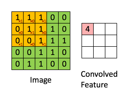
To extract features we apply Kernels to the image using the convolution operation.
A Kernel is a small matrix containing values. e.g. The following is a 3 x 3 matrix used for edge detection.

This is then passed across the image left to right, top to bottom. The values are added up into a convolved matrix or feature map. How far the Kernel is moved in each direction before we apply it is called the stride. Below shows how the convolved matrix is created using a stride of 1 pixel.
From deeplearning.stanford.edu
Code
To show the basic maths involved in a convolution i will use numpy as it has a np.convolve function.
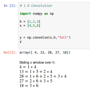
Above shows how the resulting array [4,13,28,27,18] is calculated.
Now using the same code lets see an edge detector. H is an edge detector [1,-1]. X has 2 edges where 0 goes to 1 and where 1 goes back to 0. When we convolve X and H the resulting array values are all 0s except where the two edges occur.

Image example
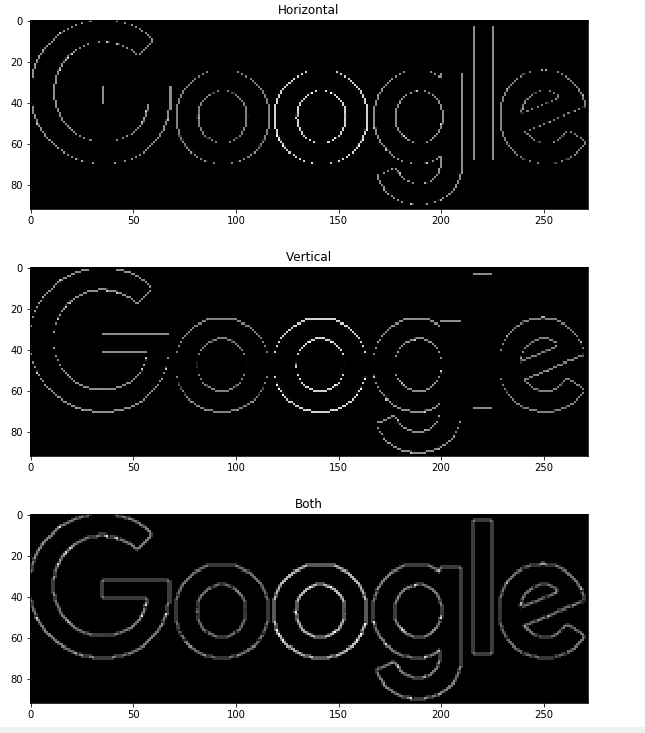
Lets apply this to a real world example – The Google logo.
Firstly download the Google image locally using wget.
#DOWNLOAD GOOGLE IMAGE

#use wget to download a local copy of google logo
!wget https://www.google.com.au/images/branding/googlelogo/1x/googlelogo_color_272x92dp.png --output-document google.png
--2017-09-23 11:11:16--  https://www.google.com.au/images/branding/googlelogo/1x/googlelogo_color_272x92dp.png
Resolving www.google.com.au (www.google.com.au)... 216.58.200.99
Connecting to www.google.com.au (www.google.com.au)|216.58.200.99|:443... connected.
HTTP request sent, awaiting response... 200 OK
Length: 5969 (5.8K) [image/png]
Saving to: 'google.png’

google.png          100%[===================>]   5.83K  --.-KB/s    in 0.003s

2017-09-23 11:11:17 (1.89 MB/s) - 'google.png’ saved [5969/5969]
Now lets display the image and convert it to grey scale and display it. Storing the image array data in imagedata.
import matplotlib.pyplot as plt
from scipy import signal
from PIL import Image

fname = 'google.png'
image = Image.open(fname)
imagedata = np.asarray(image)

plt.imshow(image)
plt.show()

imagedata = np.asarray(image.convert("L"))


plt.imshow(imagedata,cmap='gray', vmin = 0, vmax = 255)
plt.show()

Now lets create some different kernels to see their effect.
First a horizontal edge detector
# Horizontal Edge detector
kernel_horizontal = np.array([[ 0, 1, -1,0]])

convolved_horz = signal.convolve2d(imagedata, kernel_horizontal, mode='same', boundary='symm')
Second a vertical edge detector
# Vertical Edge detector
kernel_vertical = np.array([
                        [ 0],
                        [ 1],
                        [ -1],
                        [ 0]
                        ])

convolved_vert = signal.convolve2d(imagedata, kernel_vertical, mode='same', boundary='symm')
Then a more general edge detector that works both vertical and horizontal.
# Both
kernel_both = np.array([
                        [ 0, 1, 0],
                        [ 1,-4, 1],
                        [ 0, 1, 0],
                                     ])

convolved_both = signal.convolve2d(imagedata, kernel_both, mode='same', boundary='symm')
We use convolve2d from scipy instead of convolve from numpy to work in 2D.
Then lets display the results.
%matplotlib inline

fig,aux = plt.subplots(figsize=(10, 10))
aux.imshow(np.absolute(convolved_horz), cmap='gray')
plt.title('Horizontal')


fig, aux = plt.subplots(figsize=(10, 10))
aux.imshow(np.absolute(convolved_vert), cmap='gray')
plt.title('Vertical')


fig, aux = plt.subplots(figsize=(10, 10))
aux.imshow(np.absolute(convolved_both), cmap='gray')
plt.title('Both')

The best example of viewing the edge detectors is in the L of Google.
Tensorflow
The same code in tensorflow is:
#PERFORM THE SAME IN TENSORFLOW

import tensorflow as tf

#Building graph

#3x3 filter (4D tensor = [3,3,1,1] = [width, height, channels, number of filters])
#92x272 image (4D tensor = [1,92,272,1] = [batch size, width, height, number of channels]

kernel = np.array([
                        [ 0, 1, 0],
                        [ 1,-4, 1],
                        [ 0, 1, 0],
                                     ])

filter = tf.reshape(kernel.astype(np.float32),[3,3,1,1])
input = tf.reshape(imagedata.astype(np.float32),[1,92,272,1])


op = tf.nn.conv2d(input, filter, strides=[1, 1, 1, 1], padding='SAME')

#Initialization and session
init = tf.global_variables_initializer()
with tf.Session() as sess:
    sess.run(init)

    result = sess.run(op)
    print(result.shape)
    output = np.reshape(result,[92,272])
    print(output.shape)
Note you need to reshape the data a bit. The tf.nn.conv2D operation performs the 2D convolution. We have to specify the stride which is [1,1,1,1]. Channels are the depth of information per pixel. Colour pictures have 3 channels Red, Green and Blue, but this has 1 because its grey scale.

Next we will apply CNNs to the MNIST database